Introduction:
The Logistic Regression Model is a popular Machine Learning Algorithm used for Classification problems. Thus, Logistic Regression can be used to predict the risk of developing a disease based on some symptoms of a patient. Or, an email can be classified as SPAM or NOT SPAM by Logistic Regression Algorithm. It can also be used in predicting the likelihood of a Home Owner defaulting the Mortgage.
In all these examples, we are predicting an outcome “y” which has two possible values {0,1}.
Thus, y ∈ {0,1},
where 0: Negative Class
1: Positive Class
The above Binary Classification examples can be represented optionally as below:
|
0 (Negative)
|
1 (Positive)
|
|
Email Not Spam
|
Email is Spam
|
|
The HomeOwner will NOT default on Mortgage
|
The HomeOwner will default on Mortgage
|
|
The Patient will NOT develop the disease
|
The Patient will develop the disease
|
For the Binary Classification problems, the hypothesis has to satisfy the below property:
0 ≤ hθ(x) ≤1
Thus, for the Logistic Regression Model, the Hypothesis can be represented as below:
hθ(x) = g(θTx)
where g(z) = 1/(1 + e-z), the Sigmoid Function or Logistic Function
Finally, Replacing z with the above value,
Cost Function:
Now, Let’s suppose we have a Training Set with m examples. We have an (n+1) features Vector and the outcome y has two possible values {0,1}. Our objective is to choose an optimal value for 𝛉 to get a minimum cost. Now, a vectorized representation of the cost function for the logistic regression model is as below:
J(θ) = 1/m * (-yT * log(h) – (1-y)T * log(1-h))
where h =1/(1 + e-z)
Well honestly, I do not understand yet how this Cost Function is calculated for Logistic Regression Model. But apparently, this cost function can be derived from Statistics using the “Principle of Maximum Likelihood Estimation” (MLE).
Example :
Anyway, it is enough of formulae as of now. Let’s try to solve the Logistic Regression problem in R from the Andrew Ng course for Machine Learning.
So, here goes the second exercise on Logistic Regression in R. Our objective is to build a logistic regression model to predict whether a student gets admitted into a university-based on their results on two exams. We will divide this exercise in the below steps:
- Load Data
- Plot the Data
- Create a Sigmoid/Logistic Function
- Calculate the Cost
- Create a Gradient Descent Function
- Optimization and Prediction
Let’s start with the exercise!
1. Load Data:
For this exercise, the Test Data is provided in a Text file with 3 columns and 100 records. Variables V1 and V2 refer to the scores on 2 Exams and Variable V3 refer to the Admission decision.
Let’s take a look at the Data:
2. Plot the data:
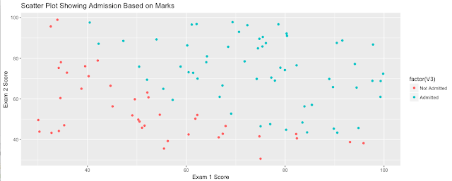
It is always advisable to visualize the data before starting to work on a particular problem. So, let’s first take a look at the data points:
Below is the plot:
3. Create Sigmoid/Logistic Function:
Let’s create the Logistic Function in R so that it can be used in the following step to calculate the Cost.
4. Calculate the Cost:
Now, we will calculate the Cost Function J(θ) with our current Dataset. Let’s create the function in R.
Now, we will test our “ComputeCost” Function. As per our current Dataset, “y” has values either 0 or 1. Initially, we will consider Theta as all zeroes.
Thus, the Cost is calculated about 0.693 using the initial parameters of theta(θ) i.e. all zeroes.
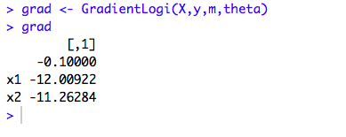
5. Calculate Gradient Descent:
Next, we will create a Gradient Descent Function to minimize the value of the cost function J(𝛉). We will start with some value of 𝛉 and keep on changing the values until we get the Minimum value of J(𝛉) i.e. best fit for the line that passes through the data points. General Form of Gradient Descent equation is as below:
Repeat{θj:=θj−αm∑i=1m(hθ(x(i))−y(i))x(i)j}
|
par
|
Initial values for the parameters to be optimized over.
|
|
fn
|
A function to be minimized (or maximized), with the first argument the vector of parameters over which minimization is to take place. It should return a scalar result
|
|
…
|
Further arguments to be passed to fn
|
|
par
|
The best set of parameters found.
|
|
value
|
The value of fn corresponding to par.
|
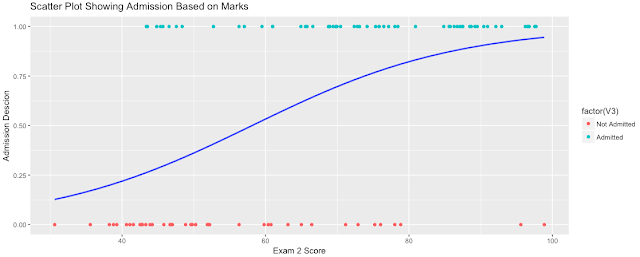
The Optimal theta is calculated as {-25.16, 0.206, 0.201} and the minimum Cost J(𝛉) at this theta value is calculated as 0.203.


