Introduction:
A Multivariate Linear Regression Model is a Linear approach for illustrating a relationship between a dependent variable (say Y) and multiple independent variables or features(say X1, X2, X3, etc.).
Univariate Linear Regression:
I had started with a simple example of a univariate linear regression model where I was trying to predict the price of the house (Y) based on the area of the property (X). Mathematically, a univariate linear regression model is represented as below:
Y = h(𝛉) = 𝛉0 + 𝛉1X
Y = output variable/target variable(SalePrice of the house)
X = input variable(LotArea of the house)
𝛉0= the Intercept
𝛉1= the slope
Multivariate Linear Regression:
Let’s extend the linear model for multiple features. Thus, a multivariate linear regression model can be represented as below:
Y = h(𝛉) = 𝛉0 + 𝛉1X1 + 𝛉2X2 + 𝛉3X3 + 𝛉4X4… 𝛉nXn
where n = total number of features
x1, x2 …xn are the different features
Y is the value to be predicted.
For simplifying the notations, let’s consider we have another feature/variable X0 and this X0 = 1 for all the values in the dataset. Thus the above equation can be written as below since X0 = 1:
Y = h(𝛉) = 𝛉0X0 + 𝛉1X1 + 𝛉2X2 + 𝛉3X3 + 𝛉4X4… 𝛉nXn
Thus, all the features can be represented by an n+1 dimensional Feature Vector X like the below one:

And all the parameters can be represented by an n+1 dimensional Parameter Vector 𝚹:

Now, we can use the concept of Transpose of a Vector, and thus the Transpose of the above Vector 𝚹 is as below:
θT =[θ0 + θ1 + θ2 +θ3 +…+θn]
Finally, a Multivariate Linear Regression Model can be expressed like:
Y = h(𝛉) =θTX
where X is the Feature Vector and θT is the Transpose of the parameter vector.
Cost Function:
As we know, in a linear regression model, we need to find out the line that fits best with our current data set. To get the best fit for this line, we need to choose the best values for 𝛉1 and 𝛉2, 𝛉3, 𝛉4 … 𝛉n and so on. Thus, we can measure the accuracy of our prediction by using a cost function J(𝛉1,𝛉2,𝛉3…𝛉n).
J(θ0,θ1…θn) = 1/2m∑ (hθ(x(i)) – y(i))2
(θ0,θ1…θn) is an n+1 dimensional Parameter Vector
m = Total Number of examples in the DataSet.
hθ(x(i)) = predicted value for the ith data and can be represented as ŷ
So, the above Cost Function can be represented simply as below:
J(𝚹) = 1/2m∑ (ŷ(i) – y(i))2
where 𝚹 = a n+1 dimension vector for the parameter values
Gradient Descent:
Similar to the Gradient Descent for a Univariate Linear Regression Model, the Gradient Descent for a Multivariate Linear Regression Model can be represented by the below equation:
repeat until convergence
{
θj = θj – α * 1/m∑ (hθ(x(i)) – y(i)). xj(i)
where j = 0,1,2…n
}
Now, let’s discuss this with an example. Even in this case, I will use the dataset example of the Machine Learning course of Andrew Ng. We will implement a linear regression model with multiple variables to predict the prices of houses.
As earlier, we will divide the whole process into the below steps:
- Load Data
- Feature Scaling
- Create a Cost Function
- Create a Gradient Descent Function and Plot the Gradient Descent Results
- Check the results
Let’s start with the exercise!
1. Load Data:
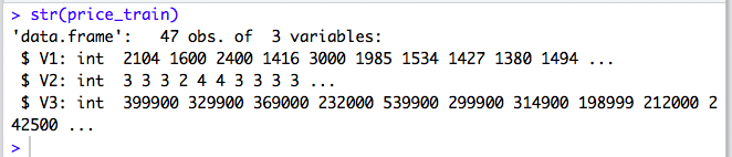
For this exercise, the Test Data is provided in a Text file with 3 columns and it contains a training set of housing prices in Portland, Oregon.
Let’s take a look at the data.
2. Feature Scaling
−1 ≤ x(i) ≤ 1 or
−0.5 ≤ x(i) ≤ 0.5
By looking at the values of our current dataset, the house sizes are about 1000 times the number of bedrooms. That’s why we will perform feature scaling and thus make gradient descent converge much more quickly. For Scaling, we will use the below Steps:
- Subtract the mean value of each feature from the dataset.
- After subtracting the mean, additionally, scale (divide) the feature values by their respective “standard deviations.”
Thus, the formula for this Feature scaling is as below:
x_norm:= xi−μisi
Where μi is the average of all the values for a feature (i) and si is the Standard Deviation.
First, let’s create a function for feature scaling using the above equation.
Then, we will call the above created function to scale our first two variables.
Let’s take a look at the scaled data:
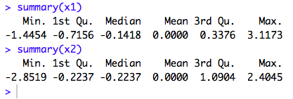
Although the values are not in the range of -1 and +1, the data is scaled to some extent.
3. Create a Cost Function:
We will create a Cost Function and will check later in the Gradient Descent function if it is converging.
4. Create a Gradient Descent Function for multiple features:
This is the step where we will create a Gradient Descent Function to get optimum values for 𝛉.
We will call the cost function created in the above step and will check if the Cost is decreasing as we are reaching the optimum parameter values.
Let’s create a Gradient Descent Function in R for multiple features.
Now, we will set alpha = 0.001 and will do 400 iterations to select the best values for 𝛉0 and 𝛉1 and 𝛉2.
Let’s take a peek at the output.
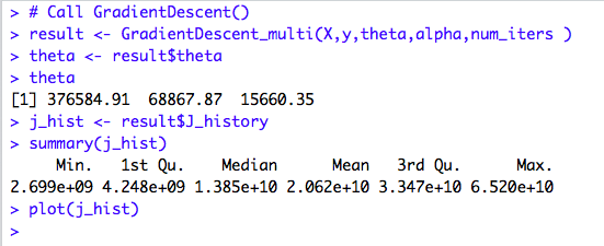
We got the below values for theta from our Gradient Descent Function:
𝛉0 = 376584.91
𝛉1 = 68867.87
𝛉2= 15660.35
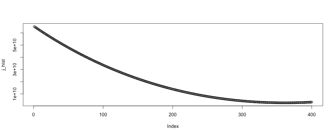
Now, let’s look at the Plot and it seems to converge.
5. Check the results
Now, as we got the values for 𝛉0 and 𝛉1 and 𝛉2, the only thing that is remaining is to check how accurate are these values of theta. So, we can predict the Sale Price for the house based on the 2 features and mathematically the Linear Model is represented as below:
Y = h(𝛉) = 𝛉0 + 𝛉1X1 + 𝛉2X2
Let’s check the results for the first data in the dataset.
The predicted value is 382035.6 and the actual value is 399900.
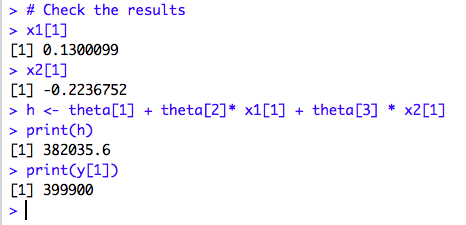
Hmmm, that means the prediction is not exact but almost accurate.
Thank You!
Unknown
good article…
Oindrila Sen
Thank You so much for pointing that out and have rectified that in my formula.
Chris Falter
Nice post. However, I think the equation for the gradient needs to be modified slightly. Instead of…
θj = θj – α * 1/m∑ (hθ(x(i)) – y(i)). x(i)
It should be, if I am not mistaken:
θj = θj – α * 1/m∑ (hθ(x(i)) – y(i)). xj(i)