Predict Your Child’s Height at 18

“Height” is a slightly delicate issue for me. I stopped growing at 5 feet. That’s why I always wonder “How Tall My Daughter Will Be @ 18?” Then one day, I asked myself, “What the Data Says”? Well, that may be an overdose of Machine Learning! But I assigned myself an exercise to predict my daughter’s height when grown up. I created my first app in Shiny and I got my answer!

Are you willing to know your’s child’s height when grown-up? Well, here is my App PredictHeight.

What is the logic behind the App? How does the Linear Regression Model look like? Welcome to the Backend story of my App “PredictHeight”. Let’s have some “serious” fun with the Data!

I will divide the whole task in the below steps.

1. Load Data
2. Visualize Data
3. Create a Linear Regression Model
4. Prediction
5. Cost Function and Gradient Descent
6. Optimization

1. Load Data:

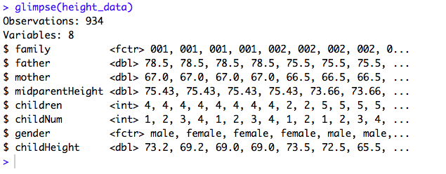
While browsing through the Internet, I got one inbuilt R dataset, named “GaltonFamilies”. It is part of the “HistData” package. Let’s Load the data and take a look!

The current Dataset has 934 observations and 8 features. Perfect!

2. Visualize Data:

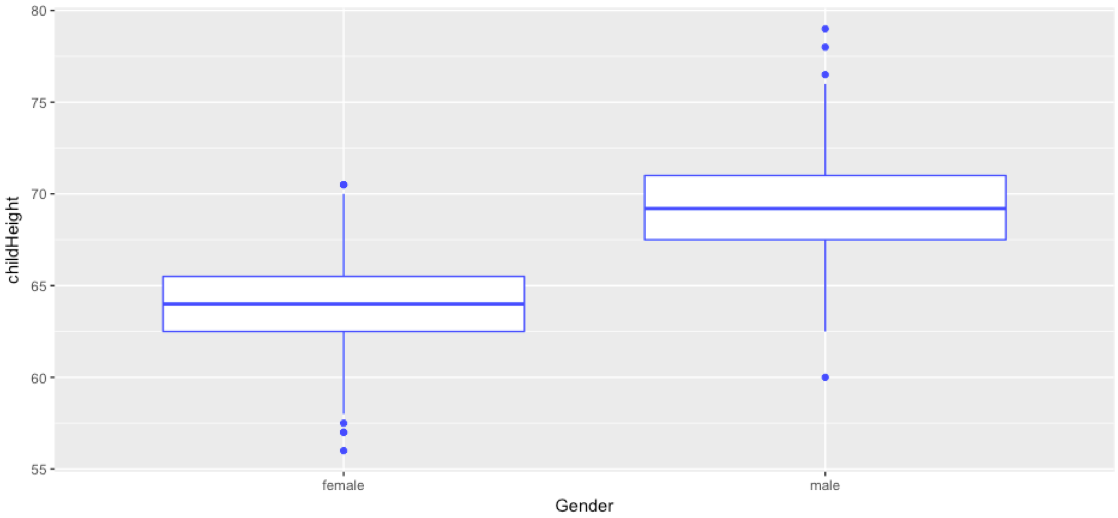
Before starting with the exercise, it is always a good idea to take a look at the Data.

Hmmm, so the data shows that on average boy height is more than a girl height.

Now, we will check the output of the average parent’s height versus a child’s height.

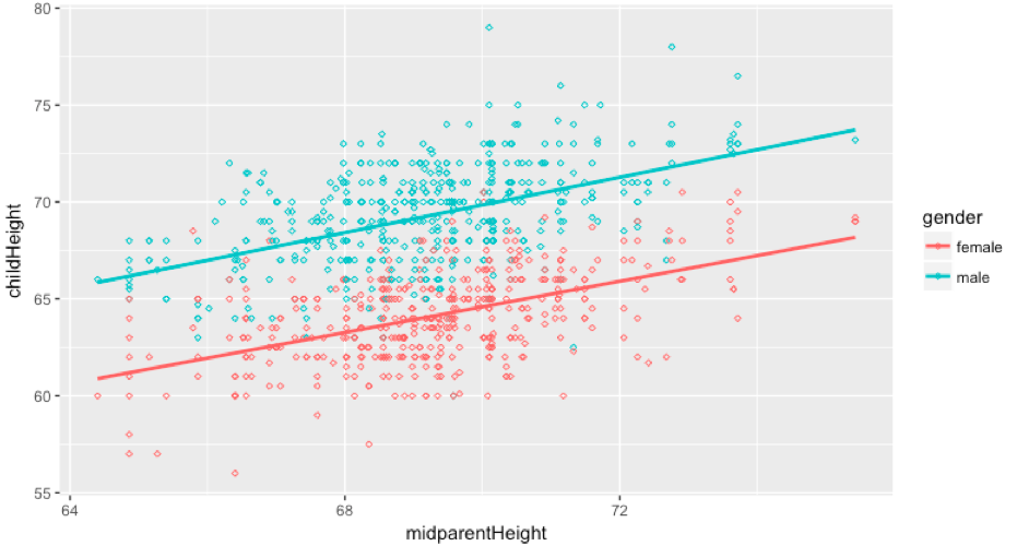
Boys are more likely to be taller than Girls. Okay, I can live with that!

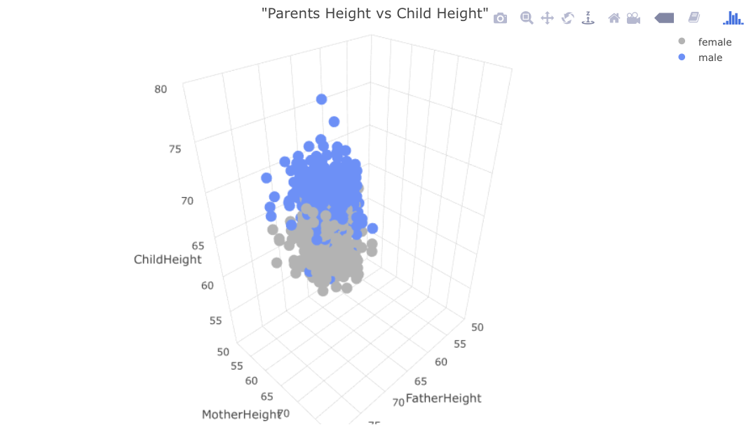
Now, let’s try a 3D plot. Well, the below plot is just an image. This is a 3D interactive plot and looks much cooler live.

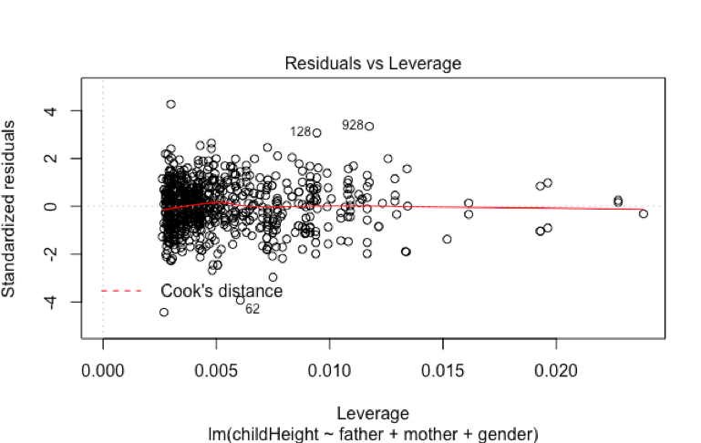
3. Create a Linear Regression Model:

For this section, first I will divide the dataset into training and test set.

Also, I need to know how accurate is the prediction.  For that, I will pass the Training Set to the Model and will test the prediction on the Test Dataset.

I think the “number of children” feature cannot affect the height of another child. So, let’s consider Father’s Height, Mother’s Height, and the Gender of the Child for the Model.

Let’s take a look at the Summary of the Model.

It seems like the features are useful and the Adjusted R Squared value is 0.6328.

4. Prediction:

Now, we can check how accurate is the predicted height.

Hmmm, it’s not exact, but more or less the same. But again, an inch or two can make a difference!

5. Cost Function and Gradient Descent:

Now, there must be some effects of Andrew Ng. Where is the Maths in here?
Let’s check the Cost Function and the Gradient Descent Function which I had described in one of my previous posts.

First, let’s check the cost function:

Now, let’s check the Gradient Descent Function:

We will now set the value of 𝛉1 = 0 and 𝛉2 = 0 and will calculate the cost.

The cost is 2233.908 which is quite high!

Starting at 𝛉1 = 0 and 𝛉2 = 0, Gradient Descent Function is returning infinite values for theta.

6. Optimization:

Let’s try to find out some optimal values for theta using the R function “Optim”. It looks like we got the below values for theta:

But, how can we be sure that these are the optimal value for theta? Does the Cost is reduced?

Oh Yes! Now the cost is reduced to  2.44!