Laptop Battery Life Challenge is an illustration that demonstrates the importance of analyzing the data before thinking of any ML solution to the problem.
Understand the Hackerrank Problem:
Fred charges his Laptop and uses it to watch TV shows until the battery dies. He has maintained a log which includes how long he had charged his Laptop and for how long he was able to watch the shows.
Thus the input data file has 100 lines each with 2 commas separated numbers:
1. The amount of time the Laptop was charged
2. The amount of time the battery lasted
Now, Fred wants to use this log to predict how long will he be able to watch TV based on his charging time so that he can plan his activities after watching his TV shows accordingly.
Here, I will put the code that I had run in rStudio for analysis. Once the analysis was done, the code in the Hackerrank editor was quite simple.
Let’s start by loading the data first.
Work for the Solution:
# Set Working Directory
setwd("/Users/oindrilasen/WORK_AREA/DataScience/HackerRank/LaptopBattery")
# Input Format
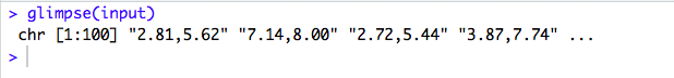
input <- readLines("trainingdata.txt", warn = FALSE)
glimpse(input)
class(input)
Let’s take a look at the data we have so far.
m = strsplit(input,split = " ")
m = unlist(m)
m
n = length(m)
n
tmp <- c()
charged_time <- c()
life_time <- c()
for (i in 1:n){
tmp[i] <- strsplit(m, split = ",")[i]
charged_time[i] <- sapply(tmp[i], "[[", 1)
life_time[i] <- sapply(tmp[i], "[[", 2)
}
charged_time <- as.numeric(charged_time)
life_time<- as.numeric(life_time)
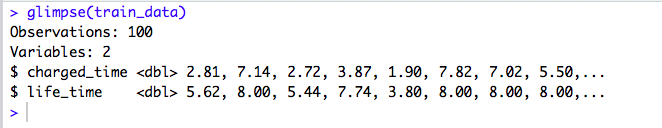
train_data <- cbind.data.frame(charged_time,life_time)
glimpse(train_data)
summary(train_data$charged_time)
summary(train_data$life_time)
There are 100 records and 2 variables. One is “charged_time” and the other one is “life_time”. We need to predict “life_time” based on the “charged_time” value.
Before proceeding any further let’s take a quick look if there is any NA’s.
Code:
# deal with NA's
sapply(train_data, function (x) sum(is.na(x)))
The data looks good. Since we have two continuous variables, I thought maybe a Linear Regression model will fit the data. I tried creating a Linear Regression Model and for the input, my predicted value was far from the expected output. So, let’s plot the data first!
Code:
# Plot data
library(ggplot2)
ggplot(train_data, aes(x = charged_time, y = life_time)) +
 geom_point() +
 geom_smooth(method = "lm") +
 scale_x_continuous(limits = c(0, 12), breaks = seq(0, 12, 1)) +
 scale_y_continuous(limits = c(0, 8), breaks = seq(0, 8, 0.8))
Here is the plot!
The simple plot shows clearly that a linear model doesn’t seem to be a good fit.
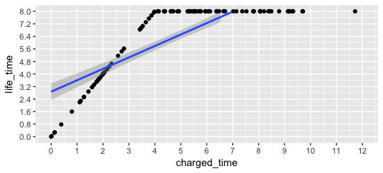
But there is a pattern in the data. If the Laptop is charged for 4 hours or more, the max life_time of the laptop is 8 hours. In other words, 4 hours can be used as a cutoff. If the Laptop is charged for less than 4 hours, the life_time seems to be directly proportional to the charged_time. But if the laptop is charged for 4 hours or more, the life_time is always 8 hours.
Here, I will divide the dataset into 2 parts. One where life_time is 8 hours and the other where life_time is less than 8 hours and then let’s take a look at how the plot looks like.
Code:
# Max life_time = 8
library(dplyr)
part1_train_data <- filter(train_data, life_time == 8)
dim(part1_train_data)
# plot
ggplot(part1_train_data, aes(x = charged_time, y = life_time)) +
  geom_point() +
  geom_smooth(method = "lm") +
  scale_x_continuous(limits = c(0, 12), breaks = seq(0, 12, 1)) +
  scale_y_continuous(limits = c(0, 8), breaks = seq(0, 8, 0.8))

 # Max life_time < 8
part2_train_data <- filter(train_data, life_time < 8)
dim(part2_train_data)
ggplot(part2_train_data, aes(x = charged_time, y = life_time)) +
  geom_point() +
  geom_smooth(method = "lm") +
  scale_x_continuous(limits = c(0, 12), breaks = seq(0, 12, 1)) +
  scale_y_continuous(limits = c(0, 8), breaks = seq(0, 8, 0.8))
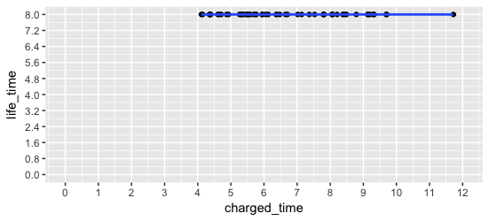 |
| Life_time is 8 hours |
 |
| Life_time is less than 8 hours |
Now, look at those plots! We don’t need any ML model to predict the life_time. A simple mathematical function is enough! If the charged_time is 4 hours or more, the life_time is a fixed value of 8 hours. If the charged_time is less than 4 hours then the life_time is 2 times the charged_time. Well, that’s it!
No ML Model or no big fat complex coding is required to solve this challenge. The data speaks everything.
Finally, The code that we need to run at Hackerrank is as below:
Thank You for reading!