First Song Recommender Model using GraphLab Create

I am introduced to GraphLab Create in Machine Learning Foundation Course by Washington University in Coursera and it is truly an amazing find. 
Let’s not go into the detailed story of its inception and rather focus on what we can do with this GraphLab Create. From my initial understanding, I assume GraphLab Create is a Tool that allows us to explore large scale data and build some advanced Machine Learning Models for predictions or recommendations or some analysis and can also help to deploy the Models in production as a Real-life Application. 

Well, I am thinking of trying my hands on some Recommender System for some time. But the concepts and Modelling is quite challenging. 
Let’s find out if GraphLab can make our life any simpler.

import sys
sys.path
sys.path.append('/Users/oindrilasen/anaconda/envs/gl-env/lib/python2.7/site-packages')
import graphlab

songs = graphlab.SFrame.read_csv("https://static.turi.com/datasets/millionsong/song_data.csv") 
usage_data = graphlab.SFrame.read_csv("https://static.turi.com/datasets/millionsong/10000.txt", 
 header=False, 
 delimiter='t', 
 column_type_hints={'X3':int})

3. Explore Data:

Now, as the data is loaded, let’s check the following:
1. how many records are there in the “songs” dataset.
2. what data is there in the “songs” dataset
3. how many records are there in the “usage_data” dataset
4. how the “usage_data” dataset look like
5. Rename the columns of “usage_data” dataset

Code 3:

len(songs) 
songs 
len(usage_data) 
usage_data 
usage_data.rename({'X1':'user_id', 'X2':'song_id', 'X3':'listen_count'})

So, there are 1 million songs data and 2 million usages. Well, that’s some huge data.

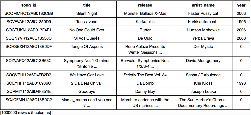Songs Data

Usage Data

4. Data Manipulation:

At the first look at song data, it shows that some songs’ year value is 0. So, how the data look like year wise?

Code 4a:

songs['year'].sketch_summary()

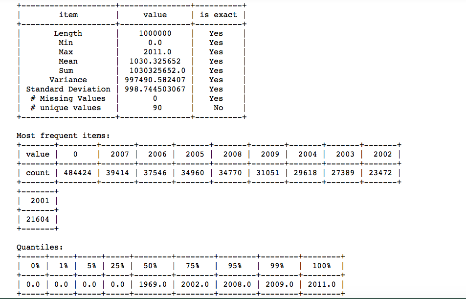
It looks like for almost half of the records, the year is “0”. And for the other half, the year ranges from 2001 to 2007. How is the year gonna modify the recommendation?

Well, it is possible that some people grew up listening to 90’s music and thus they love 90’s music. Well, that way the year can play an important role. But in this dataset, I have no way to determine the year of the songs. Besides, I don’t want to remove the records where the year is “0” because I will lose most of the Data in that case. So, let’s concentrate on some other features for a recommendation and not the year. 

Now, for any recommendation, we need to merge the two datasets first. First, let’s use an inner join to merge the two data sets and then remove the ‘year’ column since we are not going to use that.

Code 4b:

songs_usage = songs.join(usage_data, 'song_id', 'inner') 
len(songs_usage) 
songs_usage.remove_column('year')
songs_usage = songs_usage.sort('listen_count', ascending= False) 
songs_usage.head(2)

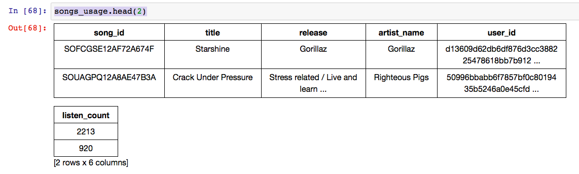
For the song “Starshine” by “Gorillaz”, the listen_count is maximum for some user and its 2213. Let’s see how popular is Gorillaz among other users. 

Code 4c:

Gorillaz = songs_usage[songs_usage['artist_name'] == 'Gorillaz'] 
len(Gorillaz['user_id'].unique()) 
len(songs_usage['user_id'].unique())

popular_artist = songs_usage.groupby(key_columns='artist_name', operations={'total_count': graphlab.aggregate.SUM('listen_count')}) 
popular_artist.sort('total_count', ascending = False)

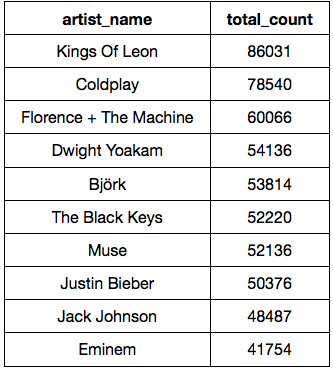
“Kings of Leon” is the most popular artist and then followed by “Coldplay”.

5. Song Recommender Model:

We can play more with the data like finding out the popular songs or release or user-wise popularity etc. But, for the time being, let’s wrap it up and start building some song recommender models.

In this section, let’s do the following:

1. Split the data into training and test set

2. Create our first recommender model based on popular artists. This is not a personalized model and it will just display the artists that are trending now.

train_data,test_data = songs_usage.random_split(.8,seed=0)
popularity_model = graphlab.popularity_recommender.create(train_data,user_id='user_id',item_id='artist_name')
results = popularity_model.recommend() 
results

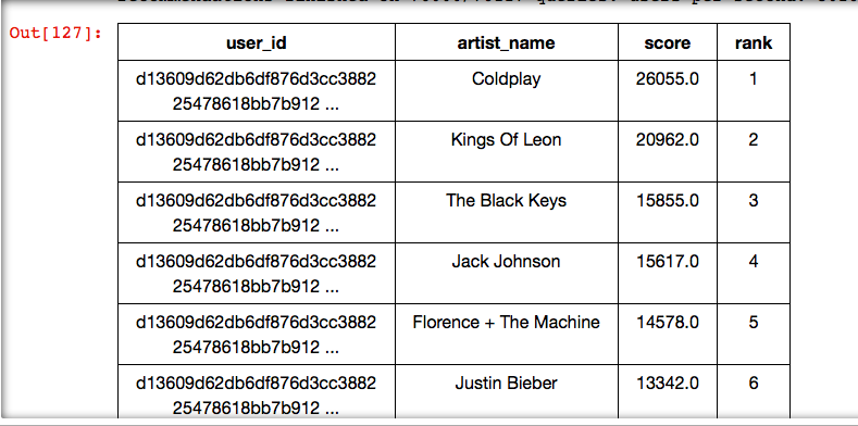
The popularity-based recommender model selects “Coldplay” at rank1 and then followed by “Kings Of Leon”. The result is not exactly the same as my simple query to select the Most Popular Artist. This model must be doing something more. But what’s remarkable here is the ease of building a Model.

 3. Let’s try a personalized model. For each user, the choices should be different. 

Code 5b:

personalized_model = graphlab.item_similarity_recommender.create(train_data, user_id='user_id', item_id='artist_name') 
users = songs_usage['user_id'].unique() 
personalized_model.recommend(users=[users[1]]) 
personalized_model.recommend(users=[users[4]])

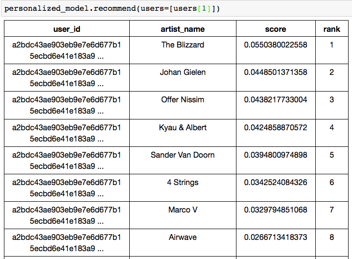
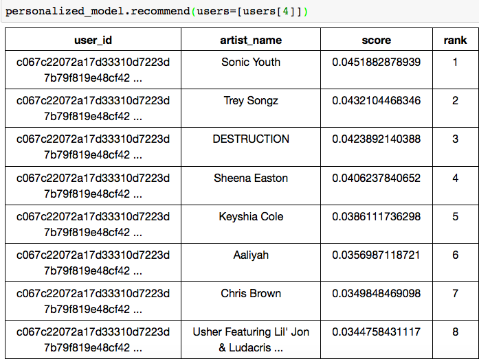
For the different users, the recommendation is different. That’s amazing. What is more amazing is how the model is created so easily by the Graphlab! We can create a similar model based on the Title of the songs. 

6. Choose a Model:

We can choose a model based on our requirements. Still, is there any way to compare the above Models and see which one has better performance?

Yes, there is a simple way!

Code 6:

model_performance = graphlab.compare(test_data, [popularity_model, personalized_model], user_sample=0.05) 
graphlab.show_comparison(model_performance,[popularity_model, personalized_model])

As per the precision-recall metric, the personalized model performed better than the popularity model.

Finally, I can also build a personalized recommender model and it is so easy! The Models were built in seconds even if the data count is huge. I am loving it! Let’s explore some more features of Graphlab as I really believe it is worth spending some more time. 


Thank You!