What is a FeedForward Neural Network?
In FeedForward Neural Network, the Perceptrons are arranged in layers, with the first layer taking in inputs (Input Layer) and the last layer producing outputs(Output Layer). Thus, the middle layers have no connection with the external world and hence are called Hidden Layers.
Each perceptron in one layer is connected to every perceptron on the next layer. Thus the information is “fed forward” from one layer to the next. There is no connection among perceptrons in the same layer.
Since the information moves in only one direction i.e. forward, from the input nodes, through the hidden nodes (if any) and to the output nodes, the Network is named as Feed-Forward Neural Network.
Mathematical Representation of FeedForward Neural Network
|
|
|
FeedForward Neural Network with One Hidden Layer
|
The above diagram denotes a simple Neural Network with one Input Layer nodes, go into another node (layer 2), which finally outputs the hypothesis function, known as the “output layer”.
The intermediate or “hidden” layer nodes a02⋯an2 are called the “activation units.”
ai(j) ->”activation” of unit i in layer j
θ(j) ->matrix of weights/parameters controlling function mapping from layer j to layer j+1
The values for each of the “activation” nodes is obtained as follows:
| a(2)1=g(Θ(1)10×0+Θ(1)11×1+Θ(1)12×2+Θ(1)13×3)a(2)2
= g(Θ(1)20×0+Θ(1)21×1+Θ(1)22×2+Θ(1)23×3)a(2)3
=g(Θ(1)30×0+Θ(1)31×1+Θ(1)32×2+Θ(1)33×3)hΘ(x)
=a(3)1=g(Θ(2)10a(2)0+Θ(2)11a(2)1+Θ(2)12a(2)2+Θ(2)13a(2)3) |
Thus, the value of each hidden activation unit (like a1(2))can be computed as Sigmoid Function applied to the linear combination of weights and input values. Now, let’s Vectorize the above equations. A new variable zk(j)can be defined that encompasses the parameters inside the g function. Thus, if we replace by the variable z for all the parameters we would get:
| a(2)1=g(z(2)1)a(2)2=g(z(2)2)a(2)3=g(z(2)3) |
Then, we can rewrite the equation as:
| z(j)=Θ(j−1)a(j−1)z(j)=Θ(j−1)a(j−1) |
Finally, We get our result with:
hΘ(x)=a(j+1)=g(z(j+1))hΘ (x)=a(j+1)=g(z(j+1))
Now, that’s a lot of confusing equations. Let’s try it out with some real data.
I have used the same old Dataset from “machine-learning-ex4” from the Andrew Ng Course of Machine Learning. Let’s load the data.
1.Load data:
There are 5000 training examples where each training example is a 20* 20 pixel grayscale image of the digit. Each pixel is represented by a floating-point number indicating the grayscale intensity at that location. The 20 by 20 grid of pixels is “unrolled” into a 400-dimensional vector. Each of these training examples becomes a single row in our data matrix X. This gives us a 5000 by 400 matrix X where every row is a training example for a handwritten digit image.
The second part of the training set (y) is a 5000-dimensional vector y that contains labels for the training set.
Also, there is a set of network parameters (Θ(1),Θ(2)) already trained. These are stored in ex4weights.mat and is loaded into Theta1 and Theta2. The parameters have dimensions that are sized for a neural network with 25 units in the second layer and 10 output units (corresponding to the 10 digit classes).
Now, we will create a function for FeedForward Neural Network and will calculate the cost. But before that, we will create one Sigmoid Function which will be used in the FeedForward Function.
2. Create a Sigmoid Function:
Now, we can create a FeedForward function and will use the Sigmoid Function created above to compute hθ(x(i))k = a(3) is the activation (output value) of the k-th output unit.
3. Create A FeedForward Function:
We used the above equations to compute hθ(x(i))k.
4. Compute the Cost:
For neural networks, The cost is computed as below:
J(Θ)=−1m∑i=1m∑k=1K[y(i)klog((hΘ(x(i)))k)+(1−y(i)k)log(1−(hΘ(x(i)))k)]
|
The double sum simply adds up the logistic regression costs calculated for each cell in the output layer.
Now, the final part of the problem. Let’s call the functions created above and take a look at the results.
5. Check Results
First, we will call the Feedforward Function to compute hθ(x(i))k. Then we will check the cost using that value.
The cost is calculated as 0.02876292 as expected in that exercise.
But something is still not clear.
How did we use the Feedforward Neural Network for our Multi-class classification problem?
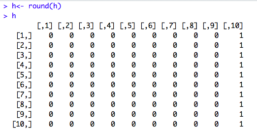
If we check the class of h computed above, it is a Matrix of 5000*10 dimension.
So, in this problem, we are trying to recognize 10 digits and thus the output h has 10 output classifiers. For each record, we can check if the output digit is for 1 or 2 or 3 and so on.
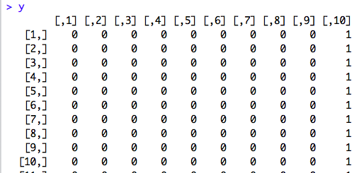
Thus, for the first 10 records, there is 1 at 10 and the rest are 0. That means, as per the Feedforward Neural Network, the first 10 numbers are predicted as 10. Now, let’s take a look at the actual first 10 outputs.
So, it looks like the prediction is correct for the first 10 records. Now, let’s take a look at the overall accuracy.
Hmm, the prediction is not 100% accurate, but not that bad either.
Thank You!
0


