Linear Regression is a technique to predict the value of an output variable based on one or more input variable(s).
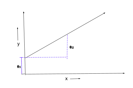
The purpose of Linear Regression is to model a continuous variable Y as a mathematical function of one or more X variable(s).A linear relationship represents a straight line when plotted as a graph and the general equation is as below:
Y = h(𝛉) = 𝛉1 + 𝛉2X
Here,
Y is the response variable (The Output variable that we are trying to predict)
X is the predictor variable (The Input Variable whose value is known)
𝛉1 is the Intercept
𝛉2 is the slope
Problem:
Solution:
1. Pick a Dataset:
| [, 1] | mpg | Miles/(US) gallon |
| [, 2] | cyl | Number of cylinders |
| [, 3] | disp | Displacement (cu.in.) |
| [, 4] | hp | Gross horsepower |
| [, 5] | drat | Rear axle ratio |
| [, 6] | wt | Weight (1000 lbs) |
| [, 7] | qsec | 1/4 mile time |
| [, 8] | vs | V/S |
| [, 9] | am | Transmission (0 = automatic, 1 = manual) |
| [,10] | gear | Number of forward gears |
| [,11] | carb | Number of carburetors |

2. Divide into Training and Test Dataset:

3. Build a Linear Regression Model:

4. Understanding the Model
Using the summary() function on the Linear Model created, we are able to see the coefficients and some other values. Let’s summarize what we can see in the above output:
1. The independent (predictor) variables are listed on the left i.e. cyl, disp, hp, etc.
2. The Estimate column gives the coefficients for the intercepts for each of the independent variables in our model.
3. The Std. Error column gives a measure of how much the coefficient is likely to vary from the estimated value.
4. The t value column is Estimate/Std Error. It is negative if the Estimate is Negative and Positive if the Estimate is Positive. The larger the ABSOLUTE value of this variable, the more likely the coefficient to be significant. So, the higher the t-value, the better.
5. The Pr(>ltl) column gives the probability that a coefficient is actually zero. We want variables with a small value in this column.
6. There is another easy way to evaluate the significance of variables by seeing the number of stars(***) at the end of each variable. But, for the above model, we are not seeing any stars for any variable.
7. After a Linear Regression Model is created, we need to determine how well the model fits the data. An important statistical measure is the R-squared value. R-squared is always between 0 and 100%:
- 0% indicates that the model explains none of the variability of the response data around its mean.
- 100% indicates that the model explains all the variability of the response data around its mean.
In general, the higher the R-squared, the better the model fits the data. But, every time we add a predictor to a model, the R-squared increases. It never decreases. That’s why it is better to check for another statistical measure the “Adjusted R-Squared” value.
8. The adjusted R-squared is a modified version of R-squared that has been adjusted for the number of predictors in the model. The adjusted R-squared increases only if the new predictor variable improves the model. It is always lower than the R-squared.
Now, let’s create another model, using a few variables with a lower value in the last column.

We can see a single star for the variables “am” and “wt”. There is a dot(.) for variable “qsec” . “hp” seems to have not much significance in building the Model. So, let’s create another model removing the variable “hp”.
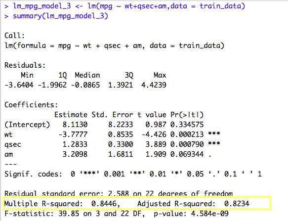
The current model, “wt” and “qsec” variable seems to have triple stars and “am” variable has a dot(.). That means, all the variables are of significant value in predicting the mpg. Also, the Adjusted R-Squared value is 0.8234 which is pretty high and thus it tells how accurate our Linear Model is.
5. Making a Prediction
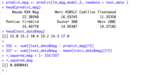
As per our Model, the Predicted mpg value for Mazda RX4 Wag is 22.30340 and the actual value in our Test dataset is 21.0 which is not exact but almost accurate. To test the accuracy of our Linear Regression Model, we can calculate the R-Squared value on our Test Data. The formula is
1- SSE/SST
In our case, the value is 0.89 which is pretty high and almost accurate.
6. Build a Mathematical Equation:

mpg = 8.1130 – (3.7777)*wt + (1.2833)* qsec + (3.2098) * am
 Lets, consider the 1st data in the Training DataSet i.e. Mazda RX4 Wag.
Let’s Calulate:
mpg(Mazda RX4 Wag) = 8.1130 – (3.7777)*2.875 + (1.2833)*17.02 + (3.2098) * 1 = 22.30368
As per the Test Data, the actual mpg value is 21.0 and the predicted value is 22.3.
The mathematical representation of a Linear Regression Model is posted here in detail.