Random Forest is a popular algorithm for Machine Learning which can be used both for Regression and Classification tasks. The concept (definition) of this algorithm is explained in its name itself.
Forest – It develops a forest with lots of decision trees.
Random – For building the decision trees, the Data is selected on random and even the variables are selected at random, each time. So, each subset can have different sizes or elements or variables and the subsets can overlap or may not overlap with each other.
In Classification problems, to determine the class of an object, a vote from each of the decision trees is considered and chooses the one with most votes.
In Regression problems, the average of the outputs from all of the different trees is considered for prediction.
Applications of Randon Forest Algorithm:
Stock Market: In the stock Market, Random Fores Algorithm can be used to identify Stock Behaviour. It can be used to predict expected loss or gain on purchasing a particular stock.
E-commerce: In- E-commerce, Random Forest can be used in recommending the customers based on similar kinds of searches.
Now, let’s start with a simple example of the Random Forest Algorithm.
Problem:
Solution:
install.packages("randomForest")
1. Pick a Dataset:
|
Variable
|
Definition
|
Values
|
|
survival
|
Survival
|
0= No, 1 = Yes
|
|
pclass
|
Ticket class
|
1= 1st, 2= 2nd, 3= 3rd
|
|
sex
|
Sex
|
Male/Female
|
|
Age
|
Age in years
|
|
|
sibsp
|
No of siblings/spouses aboard the Titanic
|
|
|
parch
|
No of parents/children aboard the Titanic
|
|
|
ticket
|
Ticket number
|
|
|
fare
|
Passenger fare
|
|
|
cabin
|
Cabin number
|
|
|
embarked
|
Port of Embarkation
|
C = Cherbourg,
Q = Queenstown,
S = Southampton
|
2. Load Data:
First, we will Load the “Train.csv” and “Test.csv” Datafiles using the function read.csv(). While loading the Datafiles, we will use na.strings = “” so that the missing values in the data are loaded as NA.We will bind these 2 Datasets into one for further Data Cleaning.
3. Data Cleaning:
To keep this example simple, we are not going to add any new features. We will do the following cleanups instead:
- Remove a few variables which may not be beneficial for our analysis.
- Check for the NA values and replace the NA values with some meaningful data.
4. Create the Model:
To create our first Random Forest Model, we need to divide the dataset into Train and Test as we did earlier. We will use randomForest() function for this example.
If we follow the above steps and try to create our first Random Forest Model, we may get an error “NAs introduced by coercion” like below:
This error occurs if there is be any variable in the Dataset with class ‘char’. Please check here for the solution.
5. Understand the Model:
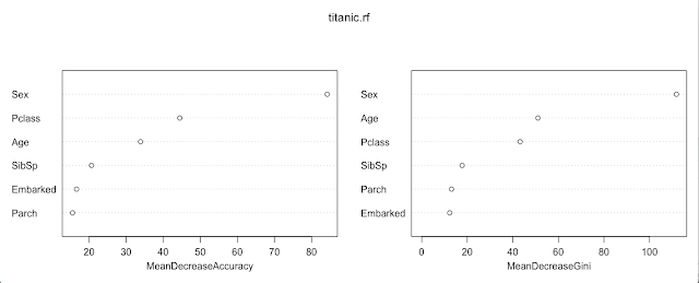
Once, the Random Forest Model is developed without any error, we can see analyze our current Model.
Meaning of the parameters used above in the Model:
Importance: Should importance of predictors be assessed?
Proximity: Should proximity measure among the rows be calculated?
ntree: Number of trees to grow
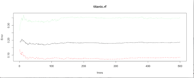
So, the output shows that it is a Classification Model and Number of variables that were tried at each split is 2. If we check the Plot, the error is gradually getting stable after 100 trees are iterated.


