Calculate Cost Function and Gradient Descent for Univariate Linear Regression in R

I was trying to follow the Machine Learning class of Andrew Ng and was soon got overwhelmed with all the mathematical representations and the equations. I decided to take small baby steps and understand the concepts first and then try out the same in R.

So, here goes the first exercise on Linear Regression with one variable in R. Here, we will predict the profits of a food truck based on the population of the cities.

We will divide this exercise in the below steps:

1. Load Data
2. Plot the Data
3. Create a Cost Function
4. Create a Gradient  Descent Function
5. Plot the Gradient Descent Results

Let’s start with the exercise!

1. Load Data:

For this exercise, the Test Data is provided in a Text file with 2 columns and 97 records. x refers to the population size in 10,000s and y refers to the profit in $10,000s.

Let’s take a look at the data structure.

2. Plot the data:

Let’s first visualize the data and try to fit in a line through the data.

Below is the plot:

3. Create a Cost Function:  

As we already know, a linear regression model is represented by a linear equation like below:
Y = h(𝛉) = 𝛉1 + 𝛉2X
Y = output variable/target variable(Profit)
X = input variable(Population)
m = number of training examples(in this example, it is 97)

We need to find out the line that fits best with our current data set. To get the best fit for this line, we need to choose the best values for 𝛉1 and 𝛉2. We can measure the accuracy of our prediction by using a cost function J(𝛉1,𝛉2). At this step, we will create this Cost Function so that we can check the convergence of our Gradient Descent Function. The details on the mathematical representation of a linear regression model are here. The equation for the cost function is as below:

J(θ0,θ1)=12m∑i=1m(y^i−yi)2

Let’s create the cost function  J(𝛉1,𝛉2) in R.

First, we will set the value of 𝛉1 = 0 and 𝛉2 = 0 and will calculate the cost.

Thus, the value of the cost J(0,0) is 32.07273.

4. Create a Gradient Descent Function:

Next, we will create a Gradient Descent Function to minimize the value of the cost function J(𝛉1,𝛉2). We will start with some value of  𝛉1 and 𝛉2 and keep on changing the values until we get the Minimum value of J(𝛉1,𝛉2) i.e. best fit for the line that passes through the data points. Gradient Descent equation for a linear regression model is as below:

Rpeat until convergence: {θ0:=θ1:=}θ0−α1m∑i=1m(hθ(xi)−yi)θ1−α1m∑i=1m((hθ(xi)−yi)xi)

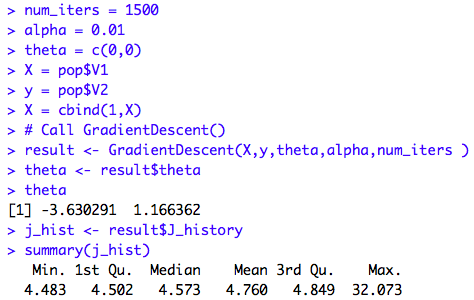
Now, we will set alpha = 0.01 and will do 1500 iterations to select the best values for 𝛉1 and 𝛉2.

Thus, the function returns the value for 𝛉1= -3.6303 and 𝛉2 = 1.1664. If we check the Cost Function (J), the value varies from 4.483(min) to 32.073(max).

5. Plot the Gradient Descent Results:

Let’s visualize how the cost function converges.

Thus the Cost Function J(𝛉1,𝛉2) is converging until we are getting the minimum value for J(𝛉1,𝛉2).

Thank You!

1