It is high time now that I slide my feet in the vast ocean of Neural Network. I was avoiding it for some time. In the first place, I wanted to use a Neural Network for the Hand-Written Digit Recognition problem. Instead, I tried the below:
3. Multinomial Logistic Regression
In this post, I will implement a simple Neural Network to recognize the handwritten digits.
I will use the same dataset from the Neural Network Exercise of the Andrew Ng Course of Machine Learning. I converted the .mat file to a .csv file. The steps are mentioned in another post here.
The inputs are pixel values of digit images. Since the images are of size 20×20, this gives us 400 input layer.
The first few steps are the same as in my last few posts and thus copy-pasted from before.
So, Let’s divide the whole process into the below steps:
- Load Data
- Divide Data into Training and Test Set
- Exploratory Data Analysis
- Create a Model
- Prediction
1. Load Data:
I have used the Dataset from “machine-learning-ex4” from Andrew Ng ‘s Machine Learning Course. I converted the .mat files to a .csv files. Let’s load the data first and take a look.
Now, let’s see what we are doing in the above piece of code.
- Load 2 data files: We have 2 data files. The first data file has 5000 training examples, where each training example is a 20 * 20 (400) pixel grayscale image of a digit. Thus, each pixel is represented by a floating-point number indicating the grayscale intensity at that location. The 20 by 20 grid of pixels is “unrolled” into a 400-dimensional vector. The second data file is a 5000-dimensional vector y that contains labels for the training set.
- Merge the 2 Datafiles: I have loaded both the datasets and merged them into a single file. Let’s check the dimension of each file.
- Rename the “output” column: The output file column name is “V1”. Also, the pixel value dataset has a column named “V1”. So, I renamed the output file column to “Output” to avoid any confusion.
- Create the Output Matrix: This step is new to this particular Neural Network Model. I am adding a 10 new columns (For number 1 to 10) and named them as “out.1”, “out.2”, “out.3” etc. and putting “1” for the value in the “output” column and “0” for the rest. i.e. If the “output” column has a value “5”, we will have a “1” in “out.5” and “0” in “out.1″,”out.2” , “out.3” , “out.4”, “out.6” , “out.7”, “out.8”, “out.9” and “out.10”. Now, if we check the dimension of the “digits” data frame, it has 411 columns.

If we check the column names, below is the list of columns:
2. Divide Data into Training and Test Set:
At this step, we will divide the dataset into the Training and Test set. We will use 70% of the data for training our Model and the other 30% to test the accuracy of our Model.
3. Exploratory Data Analysis:
This is a fun and colorful part. Let’s plot!
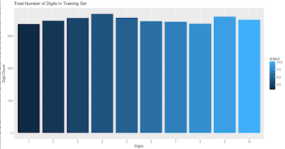
It’s time to find out how our Training Set looks like.
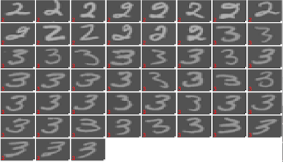
Hmm, all the digits are almost equally distributed in the Training Dataset. Now, we will see how the handwritten Digits in our training set looks like. We have created a function for the same and passed a few records randomly and below is the output.
4. Create a Model:
We will use Neuralnet for this classification problem. Let’s build a Model!
Now, let’s understand the Model First.
|
Arguments
|
Meaning
|
|
formula
|
a symbolic description of the model to be fitted.
|
|
hidden
|
integer specifying the number of hidden neurons (vertices) in each layer.
|
|
data
|
a data frame containing the variables specified in the formula.
|
|
linear.output
|
logical. specify whether we want to do regression i.e. linear.output=TRUE or classification i.e. linear.output=FALSE
|
|
algorithm
|
a string containing the algorithm type to calculate the neural network. ‘rprop+’ refers to the resilient backpropagation with weight backtracking,
|
|
learningrate
|
a numeric value specifying the learning rate used by traditional backpropagation.
|
|
rep
|
the number of repetitions for the neural network’s training.
|
For some reason, neuralnet does not like the formula y~. That’s why we have to build a formula where output variables are on the left-hand side of ~ and the predictor variables are on the right-hand side. Also, the Model will take some time to build for the first time.
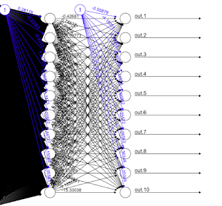
The plot with 10 hidden Units was taking some time to load and also became quite extensive. So, I changed the Hidden =1 and built the model again and plot the results.
5. Prediction:
Let’s see how the Neural Network Model performs on the test data.
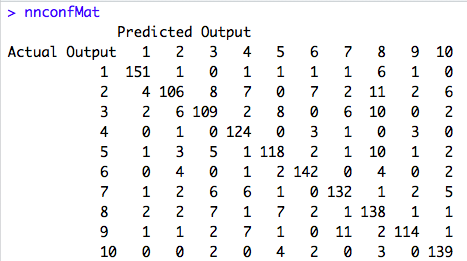
It looks like the prediction is almost 85% accurate which is not bad! Now, finally, let’s take a look at the confusion Matrix.
The Neural Network Model performed well. But for me, Random Forest is still the winner!
Thank You!


