
In this post, I will discuss the basic data science concepts that we may know but fail to express during an interview.
Let’s get started with some basic concepts of Data Science!
Let’s practice well and then keep the answers interview-ready!
1. Supervised Machine Learning:
Supervised learning is when we have a labeled dataset. If we have input variables (X) and an output variable (Y) and we use an algorithm to learn the mapping function from the input to the output [Y = f(X)], it is called supervised learning.
The aim is to approximate the mapping function so that when we have new input data (Test Data) we can predict the output variables for that data. Since we have labeled data for training, we know the correct answers. The algorithm iteratively makes predictions on the training data and on each iteration, the prediction gets closer to the actual data. Learning stops when the algorithm achieves an acceptable level of performance.
2. Unsupervised Machine Learning:
Unsupervised learning is when we have an unlabeled dataset i.e. where we only have input data (X) and no corresponding output variables. The goal of unsupervised learning is to model the underlying structure or distribution in the data in order to learn more about the data.
3. Bias-Variance Tradeoff:
The Bias-Variance Tradeoff is relevant for supervised machine learning – specifically for predictive modeling.
Bias: Bias measures the deviation between the expected output of the model and the real values, so it indicates the fit of the model.
High-Bias: Fast to learn, Easier to understand, Less flexible, Predictions are inaccurate on average. Examples: Linear Regression, Linear Discriminant Analysis, and Logistic Regression.
Low Bias: Complex Model, More Flexible, Predictions are more accurate on average. Examples: Decision Trees, k-Nearest Neighbors and Support Vector Machines.
Variance: Variance is the amount that the output of the Model will change if different training data is used.
High Variance: Suggests large changes to the estimate of the target function with changes to the training dataset. Examples: Decision Trees, k-Nearest Neighbors and Support Vector Machines.
Low Variance: Suggests small changes to the estimate of the target function with changes to the training dataset. Examples: Linear Regression, Linear Discriminant Analysis, and Logistic Regression.


The Bias-Variance Tradeoff:
If the model is too simple and has very few parameters then it may have high-bias and low-variance. On the other hand, if the model has a large number of parameters then it’s going to have high-variance and low-bias. So we need to find the right/good balance without overfitting and underfitting the data i.e. we need to find a good balance between bias and variance such that it minimizes the total error.

4. Overfitting:
Overfitting is a phenomenon that occurs when a machine learning or statistical model doesn’t generalize well from the training data to unseen (test) data.
5. Underfitting:
A statistical model or a machine learning algorithm is said to have underfitting when it cannot capture the underlying trend of the data.
6. Classification Accuracy:
It is the ratio of the number of correct predictions to the total number of input samples.
Accuracy = Number of Correct Predictions∕Total Number of Predictions
It works well only if there are an equal number of samples belonging to each class. For example, if there are 98% of samples of class A and 2% samples of class B in our training set. Then the model can easily get 98% training accuracy by simply predicting every training sample belonging to class A. When the same model is tested on a test set with 60% samples of class A and 40% samples of class B, then the test accuracy would drop down to 60%.
7. Confusion Matrix:
A Confusion Matrix gives us a matrix as output (Table layout) and describes the complete performance of the model.

8. Precision:
It is the number of correct positive results divided by the number of positive results predicted by the classifier.

Example: Email spam detection.
In email spam detection, a false positive means that an email that is non-spam (actual non-spam) has been identified as spam (predicted spam). The email user might lose important emails if the precision is not high for the spam detection model.
9. Recall:
It is the number of correct positive results divided by the number of all relevant samples (all samples that should have been identified as positive).

Example: Fraud Detection
If a fraudulent transaction (True Positive) is predicted as non-fraudulent (Predicted Negative), the consequence can be very bad for the bank.
10. F1 Score:
F1 Score is used to measure a test’s accuracy
It is the Harmonic Mean between precision and recall. The range for the F1 Score is [0, 1]. The greater the F1 Score, the better is the performance of our model

11. Root Mean Squared Error (RMSE):
RMSE is a popular evaluation metric used in Regression problems. The term is always between 0 and 1. To construct the RMSE, we first need to determine the Residuals.
Residuals: The difference between the actual values and the predicted values.

Squaring the Residuals, Averaging the squares, and taking the square root gives us the RMSE. RMSE metric is given by:

12. Imbalanced Data:
Data imbalance means an unequal distribution of classes within a dataset.
For example, in a credit card fraud detection dataset, most of the credit card transactions are not fraud and very few classes are fraud transactions. If we train a binary classification model without fixing this problem, the model will be completely biased.
Fix:
Undersampling: Randomly delete some of the observations from the majority class
Oversampling: Generate synthetic data that tries to randomly generate a sample of the attributes from observations in the minority class. The most common technique is called SMOTE (Synthetic Minority Over-sampling Technique)
13. Cross-Validation:
To evaluate the performance of any machine learning model we need to test it on some unseen data. Based on the model’s performance on unseen data we can conclude:
– our model is Under-fitting
– or our model is Over-fitting
– our model is Well generalized
Cross-Validation is a technique to evaluate the effectiveness of a machine learning model. We need to keep aside a sample /portion of Data that is not used in training the Model. This can be done in the below ways:
1. Train/ Test Split
2. Train/Validation/Test Split
3. K-fold Cross-Validation
K-fold Cross Validation Method:
Split the entire data randomly into k folds (value of k shouldn’t be too small or too high. The higher value of K leads to a less biased model (but large variance might lead to overfitting), whereas the lower value of K is similar to the train-test split approach
Then fit the model using the K-1 (K minus 1) folds and validate the model using the remaining Kth fold. Note down the scores/errors.
Repeat this process until every K-fold serves as the test set. Then take the average of the recorded scores. That will be the performance metric for the model.
14.A/B Testing
A/B testing refers to an experimental technique to compare two versions of the same webpage to determine which one performs better.
– show 50% of visitors version A (let’s call this the “Control”)
– show 50% of visitors version B (let’s call this the “Variant”)
– The version of the webpage that results in the highest conversion rate wins
15. Regression, Classification, Clustering
Regression: If the prediction value is a continuous value then it falls under the Regression type problem in machine learning. It is Supervised Learning. Example: Predicting a person’s income, or house rent, etc.
Classification: If the prediction value is a category like yes/no, positive/negative, etc. then it falls under the classification type problem in machine learning. It is also Supervised Learning. Example: Classifying an Email to be Spam or not, classifying positive or negative emotion from a review statement, etc.
Clustering: Clustering is the task of partitioning the dataset into groups, called clusters. The goal is to split up the data in such a way that points within a single cluster are very similar and points in different clusters are different. It is an unsupervised learning method.
16. Generalization Error:
In supervised learning, generalization error is a measure of how accurately an algorithm is able to predict outcome values for previously unseen data.
Generalization usually refers to an ML model’s ability to perform well on new unseen data rather than just the data that it was trained on. It is related to the concept of overfitting. If the model is overfitted then it will not generalize well.
17. Regularization:
If we have a high dimensional data set, it would be inefficient to use all the variables since some of them might be having redundant information. Also, the complexity of the Model increases, which results in increasing variance and decreasing bias i.e. overfitting.
Thus, to overcome the Overfitting problem and to help feature selection, we can use Regularization.
To do this we will introduce a penalty term to the cost function. By adding this penalty term we will prevent the coefficients of the linear function from getting too large.
Some of the Regularization techniques used to address over-fitting and feature selection are:
1. L1 Regularization
2. L2 Regularization
A regression model that uses the L1 regularization technique is called Lasso Regression.
The model that uses L2 is called Ridge Regression.
Lasso Regression (Least Absolute Shrinkage and Selection Operator) adds “absolute value of magnitude” of coefficient as penalty term to the loss function.
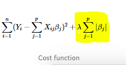
Ridge Regression adds the “squared magnitude” of coefficient as a penalty term to the loss function.
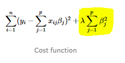
Here, if lambda is zero then we get back OLS. However, if lambda is very large then it will add too much weight and it will lead to under-fitting. Thus, it’s important how lambda is chosen.
18. Curse Of Dimensionality:
As the number of features or dimensions grows, the amount of data we need to generalize accurately grows exponentially.
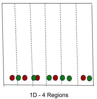
If the data points are in one dimension, that means, there is only one feature in the data set.
Now, if we add one more feature, the same data will be represented in 2 dimensions causing an increase in dimension apace to 10 * 10 = 100.

If we add 3rd feature, the dimension space will increase to 10 * 10 * 10 = 1000.

Thus, as the dimension/feature grows, dimension space increases exponentially which causes sparsity in the dataset and increases in storage space.
For example, the image recognition problem of high-resolution images 1280 * 720 pixels i.e. 921600 dimensions which are huge and unnecessary.
19. Bagging:
Bagging is an ensemble method to reduce high variance and maintaining Bias.
For Example, let us suppose there are N observations and M features.
– A sample from observation is selected randomly(with replacement).
– Then a subset of features is selected to create a model with a sample of observations and a subset of features.
– Feature from the subset is selected which gives the best split on the training data.
– This is repeated to create many models and every model is trained in parallel.
-Prediction is given based on the aggregation of predictions from all the models.
20. Boosting:
Boosting is an ensemble method for improving the model predictions of any given learning algorithm. The idea of boosting is to train weak learners sequentially, each trying to correct its predecessor.
– Build a model from the training data.
– Then build the second model which tries to correct the errors present in the first model.
– This procedure is continued and models are added until either the complete training data set is predicted correctly or the maximum number of models are added.
So, that’s all for today!
If you are preparing yourself for an interview, please check my other posts on interview preparation.
To practice python programming, you can check the challenges offered by Codility.
Below are a few solutions in python:
Keep Reading, Keep Practicing!
Thank You!
2