Let’s divide the whole process into the below steps:
- Load Data
- Divide Data into Training and Test Set
- Exploratory Data Analysis
- Create a Model
- Prediction
1. Load Data:
I have used the Dataset from “machine-learning-ex4” from Andrew Ng ‘s Machine Learning Course. I converted the .mat files to a .csv files.
Let’s load the data first and take a look.
Now, let’s see what we are doing in the above piece of code.
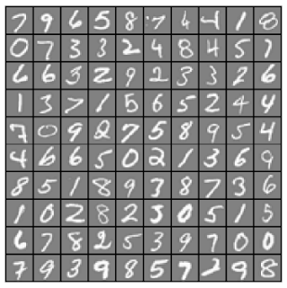
Load 2 data files: We have 2 data files. The first data file has 5000 training examples, where each training example is a 20 * 20 (400) pixel grayscale image of a digit. Thus, each pixel is represented by a floating-point number indicating the grayscale intensity at that location. The 20 by 20 grid of pixels is “unrolled” into a 400-dimensional vector. The second data file is a 5000-dimensional vector y that contains labels for the training set.
Merge the 2 Datafiles: I have loaded both the datasets and merged them into a single file. Let’s check the dimension of each file.
- Rename the “output” column: The output file column name is “V1”. Also, the pixel value dataset has a column named “V1”. So, I renamed the output file column to “Output” to avoid any confusion.
- Convert Output to a Factor column: If we check the class of the “Output” Column, it is “Integer”. Let’s Convert it to a Factor Column with 10 levels.
- Check if any column has Missing Value: I just wanted to check if there is any missing value. But it seems like there is not missing value and we are all set for the next step.
2. Divide Data into Training and Test Set:
3. Exploratory Data Analysis:
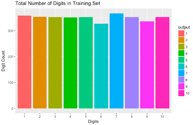
It’s time to find out how our Training Set looks like.
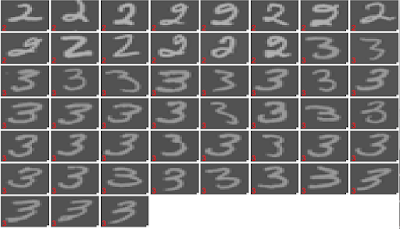
Hmm, all the digits are almost equally distributed in the Training Dataset. Now, we will see how the handwritten Digits in our training set looks like. We have created a function for the same and passed a few records randomly and below is the output.
4. Create a Model:
We will use the Decision Tree for this classification problem. We are going to use the library rpart (Recursive Partitioning and Regression Trees)for the same.
It seems like, the Model has only used a few columns for the Tree Construction.
The classification tree looks a little messed up, but still, we can get an idea that how the classification was done.
5. Prediction:
Now here is the grand finale! Let’s Test our Decision Tree Model on our Test Set by using the predict function.
Well, the number doesn’t look promising right? Now, let’s take a look at the Confusion Matrix.
The accuracy of the Model is 0.6246666667.
Now, Let’s test a number at random.
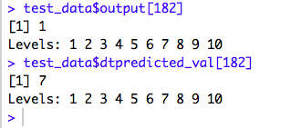
I checked the label for the 182nd row from the Test Dataset. it shows “1”. Let’s see what my Model predicted for the same. It says “7”! Okay, that’s close, but not correct!
So, how does the Handwritten Digit look like?
Hmm, that’s a tough call!
Now, we need to check some alternative Algorithms for the same and see if we can increase the Accuracy of the Prediction and that will be my next posts.
Here is the randomForest Model which proved to be a better fit.
Thank You!


Komal
very informative article post. much thanks again
Data Science Training in Hyderabad
Aditi Digital Solutions
your article on data science is very interesting thank you so much.
your article on data science is very interesting thank you so much.