Before starting my journey in Machine Learning, I knew that it would require some concepts of Mathematics. But while learning the supervised algorithms in R, I left behind the math part.
So, today let me revisit the concepts of Linear Regression with some Mathematics.
What is a Linear Regression?
By now, we understand that Linear Regression is a Supervised Learning Method where we are trying to predict some results with a continuous output i.e. we are trying to map input variables to some continuous function for prediction.
Let’s start with a simple example of Univariate Linear Regression.
So, What is a Univariate Linear Regression?
A Univariate linear regression is used when we want to predict a single output value (say y) from a single input value(say x).
Let’s consider the example of predicting house price (y) based on the area of the property(x). For this, I have taken the dataset from Kaggle for “House Prices: Advanced Regression Techniques“.
Example:
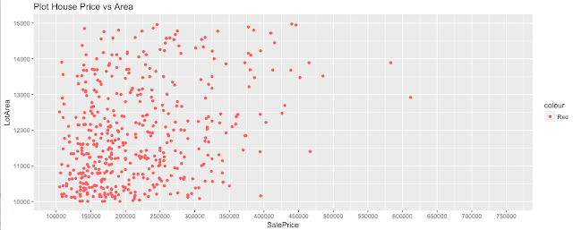
I have just loaded the Training Dataset alone and have removed all the features(variables) except LotArea and SalePrice. To keep this example a simple one, I have filtered a few records and just considering around 500 records.
Now, let’s take a look at the plot.
Well, our purpose is to build a linear regression model to predict the house price based on the area of the house. For this, we will feed our Training Data to a Learning Algorithm. The Learning Algorithm will return a function that will take an input x(LotArea) and will give an output y(SalePrice).
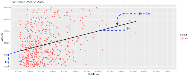
This function can be represented as below:
Thus, y is a linear function of x. Now, let’s take a look at a few records from our current dataset and try to map with our mathematical representation.

y = output variable/target variable(SalePrice of the house)
x = input variable(LotArea of the house)
m = number of training examples(in this example, it is 597)
We need to find out the line that fits best with our current data set and below is the output.
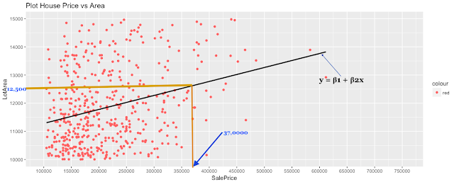
Now, if we try to predict the SalePrice of a house based on an area around 12,500 square feet, we can map the “Lotarea” on that line and predict the “SalePrice”. In this example, it is around 37,0000.
Thus, better the fit of that line, better would be our prediction.
Now, let’s try to figure out the best possible straight line with our current dataset. In other words, we need to choose the best values for 𝛉1 and 𝛉2, the parameters for the function y with a given value of x. Now, the question is “How to choose the value 𝛉1 and 𝛉2 for the best possible fit?”
The idea is we need to choose the value of 𝛉1 and 𝛉2 such that the value we predict(y) is close to the existing value y for our training example (x,y). It’s still confusing, right?
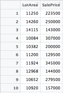
This is our data.
Here, (x1,y1) corresponds to the value (11250,223500).
Similarly, (x4,y4) is equal to (10084,307000).
Understanding the Model
If we try to think of it in a visual way, our training data set is scattered on the x-y plane. We are trying to make a straight line that passes through these scattered data points. Our goal is to get the best possible line.
The best possible line will be such that the average squared vertical distances of the scattered points from the line will be the least. Ideally, the line should pass through all the points of our training dataset.
Cost Function:
Thus, we can measure the accuracy of our prediction by using a cost function also known as “Squared error function”, or “Mean squared error” function. This takes an average difference of all the results of the hypothesis with inputs from x’s and the actual output y’s.
This cost function can be denoted as J(𝛉1,𝛉2) and can be represented as below:

where n = Total number of examples in the Training Dataset.
predi = 𝛉1 + 𝛉2 * x
yi = actual value of y
Now, if 𝛉1 = 0, predi = 𝛉2*x.
That means we will get a straight line function where the intercept is 0 i.e. a line that passes through the origin(0,0).
Example:
Calculate Cost Function:
We can try out various values of 𝛉1 and 𝛉2 to minimize J(𝛉1,𝛉2) and thus get the best possible fit or the most representative straight line through the data points of our current dataset mapped on an x-y plane.
The value of J(𝛉1,𝛉2) can be minimized if we can minimize the difference between the predicted value and the actual value.
To estimate the parameters 𝛉1 and 𝛉2 we can use the concept of Gradient Descent algorithm and thus get the best “fit” of the linear regression model.
Thank You!


